First Quarter Research Progress and Ideas

To be honest, I spent most of my first quarter of graduate school on classes, seminars, and getting adjusted to the new environment. However, I did start attending research meetings in a group I am interested in, and I have some ideas for a potential project. I am very excited about beginning this project, and I hope that this coming quarter, I will be able to make more progress. Luckily, there is a postdoc in the group who is also excited about it, and he has been very thorough in providing me with papers to read and feedback on my work. I will begin to describe my progress briefly.

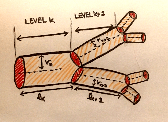
The group I have been working in studies a wide range of systems such as predator-prey dynamics, multi-drug interaction, the relationship between sleep and metabolic rate, and cardiovascular networks. Since there are so many diverse projects happening in our group, our group meetings are split by topic. The sub-group I joined focuses on networks. So far, they have been mostly focusing on cardiovascular networks. They develop models that describe these networks, such as the scaling laws that describe changes in the radius and length of vessels across levels of the network. Then, they test these models against data extracted from 3D images.

IMG_9207

Since my primary interest in biology is in neuroscience, I approached the group to find out if there were any projects in neuroscience. The PI told me that although there are currently no projects in neuroscience in this group, there are mathematical similarities between neuronal networks and cardiovascular networks, and he saw a future in extending the image analysis of cardiovascular networks to neurons.

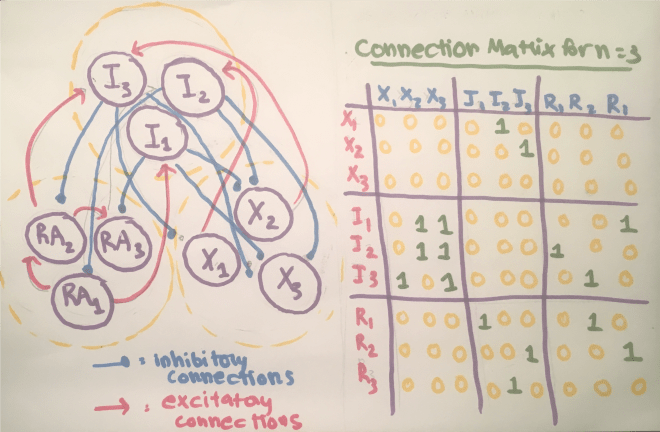
We can think of a network of neurons like the cardiovascular system, a resource distribution network that is subject to biological and physical constraints.  Deriving a power law relationship between radius and length of successive levels of a vascular network relies on minimizing the power lost due to dissipation while maintaining the assumptions that the network is of a fixed size, a fixed volume, and space filling. This calculation is carried out using the method of Lagrange multipliers, and assuming that the flow rate is constant. The power loss due to dissipation in the cardiovascular network is $P = \dot{Q_0}^2 Z_{net}$, where $\dot{Q_0}$ is the volume flow rate of blood and $Z_{net}$ is the resistance to blood flow in the network. For a neuronal network, we will use an analogous equation, $P = I_0^2 R_{net}$, where $I_0$ is the current, and $R_{net}$ is the resistance to current flow in the network. We will carry out the Lagrange multiplier calculations in a similar fashion to the calculations for cardiovascular networks.

For cardiovascular networks, we use the Poiseuille formula for resistance, which is the hydrodynamic resistance to blood flow in the network. According to this formula, the impedance at a level k in the network is given by $Z_k = \frac{8 \mu l_k}{\pi r_k^4}$. We can reduce $\frac{8 \mu}{\pi}$ to a single constant C, so this is equivalent to $Cl_k r_k^{-4}$. Thus, the resistance is proportional to the product of some powers of the length and the radius. If we want to consider a general formula for the resistance, we can consider a formula with powers p and q of of length and radius respectively. That is, our resistance formula at level k is $R_k = \Tilde{C} l_k^p r_k^q$.

We define the objective function as follows:
\[P = I_0^2 R_{net} + \lambda V + \lambda_M M + \sum_{k=0}^{N} \lambda_k n^k l_k^3 \]

This objective function arises from the fact we want to minimize power loss, the first term, while imposing the three constraints that correspond to the last three terms: size, volume, and space filling. Each constraint corresponds to a Lagrange multiplier. The last constraint comes from the fact that a resource distribution network must feed every cell in the body. This, each branch at the end of the network feeds a group of cells called the service volume, $v_N$, where N is the terminal level, and the number of vessels at that level is $N_N$, so the total volume of living tissue is $V_{tot} = N_N v_N$. If we assume that this argument holds over all network levels, we have $N_N v_N = N_{N-1} v_{N-1} = … = N_0 v_0$. We assume that the service volumes vary in proportion to $l_k^3$, so the total volume is proportional to $N_kl_k^3$. Our objective function has N terms related to space filling, since the space filling constraint must be satisfied at each level k. We assume that the branching ratio is constant, so the number of vessels at level k is $n^k$. We can define the volume as $\sum_{k=0}^N N_k \pi r_k^2 l_k$.

Note that we are defining the constraints the same we we did for vascular networks, but it is unclear whether these assumptions are accurate for neuronal networks. However, for the sake at arriving at a preliminary theoretical result for the scaling of neuronal networks, we will keep constraints.
The total resistance at each level is the resistance for a single vessel divided by the total number of vessels, that is, $R_{k, tot} = \frac{\Tilde{C} l_k^p r_k^q}{n^k}$. The net resistance of the network is the sum of the resistances at each level, so $R_{net} = \sum_{k = 0}^N \frac{\Tilde{C} l_k^p r_k^q}{n^k}$. If we define new Lagrange multipliers, $\lambda’ = \pi \lambda$, we can rewrite the objective function as follows:
\[P = I_0^2 \sum_{k = 0}^N \frac{\Tilde{C} l_k^p r_k^q}{n^k} + \lambda’ \sum_{k=0}^N n^k r_k^2 l_k + \lambda’_M M + \sum_{k=0}^{N} \lambda’_k n^k l_k^3 \]

To normalize further, we can divide by the constant $I_0^2\Tilde{C}$, since the current is constant, and absorbing this constant into new definitions of the Lagrange multipliers, we get:

\[P = \sum_{k = 0}^N \frac{l_k^p r_k^q}{n^k} + \Tilde{\lambda} \sum_{k=0}^N n^k r_k^2 l_k + \Tilde{\lambda}_M M + \sum_{k=0}^{N} \Tilde{\lambda}_k n^k l_k^3 \]

To find the radius scaling ratio, we will minimize P with respect to $r^k$, at an arbitrary level k, and set the result to 0. Thus, we can find a formula for a Lagrange multiplier and derive the scaling law.

So we have:

\[\frac{dP}{dr_k} = \frac{l_k^p qr_k^{q-1}}{n^k} + 2 \Tilde{\lambda} n^k r_k l_k = 0 \]

Solving for the Lagrange multiplier, we have:

\[\Tilde{\lambda} = -\frac{qr_k^{q-1}l_k^p}{2n^{2k} r_k l_k} = \frac{\frac{-q}{2}}{n^{2k}l_k^{1-p}r_k^{2-q}}\]

Since this is a constant, the denominator must be constant across levels. So

\[\frac{n^{2(k+1)}l_{k+1}^{1-p}r_{k+1}^{2-q}}{n^{2k}l_{k}^{1-p}r_{k}^{2-q}} = 1\]

It is useful to consider the case where the resistance is related to the length linearly, that is, for p =1. Thus, we obtain the scaling ratio:

\[\frac{n^{2(k+1)}r_{k+1}^{2-q}} {n^{2k}r_{k}^{2-q}} = 1 \rightarrow \frac{r_{k+1}}{r_k} = n^{\frac{-2}{2-q}}\]

To find the length scaling ratio, we will minimize P with respect to $l^k$, at an arbitrary level k, and set the result to 0. Thus, we can find a formula for a Lagrange multiplier, using the formula above, and derive the scaling law.

So we have:

\[\frac{dP}{dl_k} = \frac{pl_k^{p-1}r_k^{q}}{n^k} + \Tilde{\lambda} n^k r_k^2 + 3\Tilde{\lambda_k} n^k l_k^2 = 0 \]

Solving for the Lagrange multiplier, we have:

\[\Tilde{\lambda_k} = \frac{-\frac{pl_k^{p-1}r_k^{q}}{n^k} – \Tilde{\lambda} n^k r_k^2}{3n^k l_k^2}\]

Substituting $\Tilde{\lambda}$, as calculated before:

\[\Tilde{\lambda_k} = \frac{-\frac{pl_k^{p-1}r_k^{q}}{n^k} + \frac{q r_k^2}{2n^{k}l_k^{1-p}r_k^{2-q}} }{3n^k l_k^2} = \frac{(\frac{q}{2} – p)pr_k^q l_k^{p-1}}{3n^{2k} l_k^2} = \frac{q-2p}{6} \frac{1}{n^{2k}l_k^{3-p}r_k^{-q}}\]

Since this is a constant, the denominator must be constant across levels. So

\[\frac{n^{2(k+1)}l_{k+1}^{3-p}r_{k+1}^{-q}}{n^{2k}l_{k}^{3-p}r_{k}^{-q}} = 1\]

In the case where p=1, we have

\[ \frac{n^{2(k+1)}l_{k+1}^{2}r_{k+1}^{-q}}{n^{2k}l_{k}^{2}r_{k}^{-q}} = 1\rightarrow (\frac{l_{k+1}}{l_k})^2 = n^{-2} (\frac{r_{k+1}}{r_k})^q\]

Substituting the scaling law for radius, we have:
\[ (\frac{l_{k+1}}{l_k})^2 = n^{-2} (n^{\frac{-2}{2-q}})^q \rightarrow \frac{l_{k+1}}{l_k} = n^{-1 – \frac{q}{2-q}} \rightarrow \frac{l_{k+1}}{l_k} = n^{\frac{-2}{2-q}} \]

We can test these calculations for our vascular networks calculation, where q = -4. Our scaling laws for radius and length are $\frac{r_{k+1}}{r_k} = \frac{l_{k+1}}{l_k} = n^{-1/3}$, as expected.

We will now attempt to repeat these calculations using a resistance formula specific to neuronal networks.

We think of the resistance to blood flow as the resistance due to the viscosity of the fluid. For neuronal networks, we can think of axons and dendrites as wires through which current is flowing. The resistance as the resistance to current flow through the “wire” due to intrinsic properties of the wire. The resistance is given by $R_k = \frac{\rho l_k }{A}$, where A is the cross-sectional area of the wire, and $l_k$ is the length of the segment at that level. $\rho$ is the intrinsic resistivity of the axon or dendrite, and we are assuming that $\rho$ is constant, meaning that the material is uniform. If we assume that the axons or dendrites are cylindrical, we can define the cross-sectional area as $\pi r_k^2$ for level k, so the resistance for level k is given by $R_k = \frac{\rho l_k }{\pi r_k^2}$.

Assuming that the branching ratio is constant, the number of branches at each level is $n^k$, and the total resistance at each level is $R_{k,tot} = \frac{\rho l_k }{\pi r_k^2 n^k}$. The net resistance is the sum across all levels, that is $R_{net} = \sum_{k=0}^N\frac{\rho l_k }{\pi r_k^2 n^k}$.

Our objective function for this case can be derived in a similar manner as in the general case, setting $\Tilde{C} = \frac{\rho}{\pi}$, setting p = 1, and q = -2, based on the constants and powers for our specific resistance equation. Thus, we have the objective function

\[P = \sum_{k = 0}^N \frac{l_k}{r_k^2 n^k} + \Tilde{\lambda} \sum_{k=0}^N n_k r_k^2 l_k + \Tilde{\lambda}_M M + \sum_{k=0}^{N} \Tilde{\lambda}_k n^k l_k^3 \]

To find the radius scaling ratio, we will minimize P with respect to $r^k$, at an arbitrary level k, and set the result to 0. Thus, we can find a formula for a Lagrange multiplier and derive the scaling law.

So we have:

\[\frac{dP}{dr_k} = \frac{-2l_k}{n^k r_k^3} + 2 \Tilde{\lambda} n^k r_k l_k = 0 \]

Solving for the Lagrange multiplier, we have:

\[\Tilde{\lambda} = \frac{1}{n^{2k}r_k^{4}}\]

Since this is a constant, the denominator must be constant across levels. So

\[\frac{n^{2(k+1)}r_{k+1}^{4}}{n^{2k}r_{k}^{4}} = 1\]

Thus, we can solve for the scaling ratio:

\[ \frac{r_{k+1}}{r_k} = (n^{-2})^{1/4} = n^{-1/2}\]

To find the length scaling ratio, we will minimize P with respect to $l^k$, at an arbitrary level k, and set the result to 0. Thus, we can find a formula for a Lagrange multiplier, using the formula above, and derive the scaling law.

So we have:

\[\frac{dP}{dl_k} = \frac{1}{n^k r_k^2} + \Tilde{\lambda} n^k r_k^2 + 3\Tilde{\lambda_k} n^k l_k^2 = 0 \]

Solving for the Lagrange multiplier, we have:

\[\Tilde{\lambda_k} = \frac{-\frac{1}{n^k r_k^2} – \Tilde{\lambda} n^k r_k^2}{3n^k l_k^2}\]

Substituting $\Tilde{\lambda}$, as calculated before:

\[\Tilde{\lambda_k} = \frac{-\frac{1}{n^k r_k^2} – \frac{1}{n^{k}r_k^{2}} }{3n^k l_k^2} = – \frac{2}{3n^{2k}l_k^2 r_k^2}\]

Since this is a constant, the denominator must be constant across levels. So

\[\frac{n^{2(k+1)}l_{k+1}^{2}r_{k+1}^{2}}{n^{2k}l_{k}^{2}r_{k}^{2}} = 1\]

Thus, substituting in the scaling ratio for radius, we can solve for the scaling ratio for length:

\[(\frac{l_{k+1}}{l_k})^2 = n^{-2} (\frac{r_{k+1}}{r_k})^{-2} = n^{-2} (n^{-1/2})^{-2} = n^{-1} \rightarrow \frac{l_{k+1}}{l_k} = n^{-1/2}\]

Note that these scaling laws are consistent for the theoretical predictions from our general formulas, for q = -2.

Some of the assumptions we have made for the purpose of these calculations are as follows:

  • The current flow is constant across all levels of the network
  • The axons and dendrites are cylindrical
  • The material of the axons and dendrites is uniform and can be linked to a constant of specific resistivity
  • The network has a fixed size
  • The network is contained within a fixed volume
  • The network is space filling
  • The branching ratio is constant

Particularly in the case of the volume and space-filling constraints, and the constant branching ratio, it is unclear if a neuronal network has the same properties that we assume hold for vascular networks. In addition, it is unclear whether it is reasonable to assume that the current flow is constant. Thus, it might be worth reexamining these constraints and assumptions to add more biologically realistic and relevant ones.

Moreover, instead of focusing on this optimization problem of minimizing power loss, it might be more fruitful to examine a different optimization problem, such as minimizing the time for a signal to travel from one end to another end of the network.

These scaling laws give us some preliminary ideas to work with. We can try using image analysis techniques to measure length and radii of segments of axons and dendrites across levels in images and see whether information extracted from the data supports our theoretical conclusions.


References

Savage, Van M., Deeds, Eric J., Fontana, Walter. (2008). Sizing up Allometric Scaling Theory. PLOS Computational Biology.

Johnston, Daniel, Wu, Samuel Miao-Sin . (2001). Foundations of Cellular Neurophysiology. MIT Press.

Network Dynamics, Biophysics, and Mental Illness

[latexpage] This past fall was my first quarter of graduate school, and one of our core courses was Deterministic Models in Biology. For our final project, we chose a quantitative biology paper on a topic of our interest and presented on it to the class. The paper I chose was a review paper, Psychiatric Illnesses as Disorders of Network Dynamics by Daniel Durstewitz, Quentin J.M. Huys, and Georgia Koppe. My undergraduate research focused on the dynamics of neurons at the molecular level, and this paper helped me connect it to specific characteristics of mental illnesses.

This paper proposes that since observable cognitive and emotional states rely on the underlying dynamics of neuronal networks, we should use Dynamical Systems Theory (DST) to characterize, diagnose, and develop therapeutic strategies for mental illness.

The central idea of DST is that there is a set of differential equations that evolve in time. A set of dynamical equations could look as follows:

\[\frac{dx_1}{dt} = \dot{x_1} = f_1(x_1, … , x_M, t; \boldsymbol{\theta} )\]
\[\frac{dx_2}{dt} = \dot{x_2} = f_1(x_1, … , x_M, t; \boldsymbol{\theta})\]
\[\vdots \]
\[\frac{dx_M}{dt} = \dot{x_M} = f_M(x_1, … , x_M, t; \boldsymbol{\theta})\]

The variables $x_1, x_2, … x_M$ represent the dynamical variables such as voltage or neural firing rate. These equations describe how each of these variables change over time. $\boldsymbol{\theta}$ represents parameters, fixed values that are properties of the system that do not change over time.

We define a fixed point as the point at which the derivatives of all of the variables are equal to 0. Fixed points are stable if activity converges towards them, and unstable if activity diverges from them. Stable fixed points are called attractors. We can define the basin of attraction as the set of points from which activity converges towards the attractor.

The figure below shows an example of a phase plane, a representation of a space spanned by the two variables of a system. Note that it is possible to use dimensionality reduction methods to obtain visual representations for higher dimensional systems. The arrows show the activity of the system. The blue and orange curves represent nullclines, and along each of these curves, the derivative of one of the variables is 0. The green line represents the barrier between the two basins of attractions. It is possible to cross over this barrier as a result of either external influences or random fluctuations.

IMG_9208

I will discuss some basic neuroscience before going into the dynamics of mental illnesses. There are many ion currents that pass through a neuron membrane such as sodium, potassium, and calcium. The dynamics of these ions are driven by electrochemical gradients. Spiking activity occurs when there is a rapid influx of sodium ions, producing the spike followed by an efflux of potassium ions, returning the membrane potential to the threshold potential.

We can think of a neuron membrane as a capacitor, where positive and negative charges are accumulated on either side. The current is the rate of charge flowing per time, $I = \frac{dq}{dt}$, and the charge of a capacitor is defined as q = CV. The current through the membrane is this $ I_m = C_m \frac{dV_m}{dt}$. We can think of this system as the circuit shown below:

IMG_9210
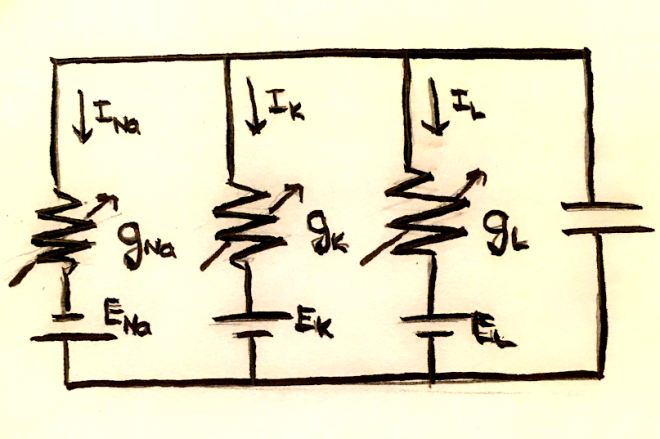
Because of charge conservation, the sum of the currents across the capacitor and each of the resistors must be 0. In mathematical terms, this is $C_m \frac{dV_m}{dt} = -\sum_i I_i$.

If we approximate each of these currents as ohmic, they will satisfy Ohm’s law, V = IR, meaning that the current is proportional to the difference between the membrane voltage and the threshold voltage by a factor of 1/R, or in other words, the conductance.

If the conductance were constant over time, these would be linear. However, the conductance depends on the proportion of ion channels that are open and the proportion of channels that are closed, called the gating variables. For example, a sodium current can be described as

$I_{Na} = g_{max}m^3h(V_m – E_{Na})$

In this system, m and h are the gating variables, and they vary from 0 to 1, and $g_{max}$ is the maximal conductance.

We can think of the dynamical equations for the gating variables as the result of a mass equation. Consider the reaction

$Closed \rightleftharpoons Open $

Suppose $\alpha$ is the rate of opening of a channel, or the forward reaction above, and $\beta $ is the rate of closing, the reverse reaction above, and both of these rates depend on the voltage. If m represents the proportion of channels that are open, the derivative over time is equal to the  forward rate times the concentration of reactants minus the reverse rate times the concentration of products. In other words:

$\frac{dm}{dt} = \alpha(V_m)(1-m) – \beta (V_m)m$

Another form of this dynamical equation commonly seen in the literature is:

$\frac{dm}{dt} = \frac{m_{\infty}(V_m) – m}{\tau_{Na}(V_m)}$

$\tau_{Na}$ is the voltage-dependent time constant, and $m_{\infty}$ is the steady-state proportion of open channels as a function of voltage.

The dynamical equation for voltage for the simple NaKL model is as follows:

\[\frac{dV}{dt}
= g_{Na}m^3h(E_{Na}-V) + g_K n^4 (E_K -V) + g_L (E_L – V) + I_{inj}C^{-1}\]

Neuronal networks are the result of multiple neurons connected to one another through synapses. Pre-synaptic neurons deliverer chemicals, called neurotransmitters, to post-synaptic neurons. Some neurotransmitters are excitatory, such as NMDA (N-Methyl-D-aspartic acid), meaning they increase the likelihood of spiking activity, and others are inhibitory, such as GABA (gamma-aminobutyric acid), meaning that they decrease the likelihood of spiking activity. To describe the networks of neuronal networks, each individual neuron has a voltage equation as illustrated above, with additional terms relating to its synaptic currents. These currents depend on the synaptic conductance, the difference between the membrane voltage and the threshold voltage, the strengths of the synaptic connections, and the fraction of open channels for each receptor. The dynamical equation for the fraction of open channels usually depends on properties of the presynaptic neuron.

So far, the variables we have been considering have been the voltage and the gating variables. In order to discuss the dynamics of mental illness, we must think about another important variable: firing rate. This simply describes the rate of voltage spikes over time. Below is an example of a phase plane, where the vertical axis is the average firing rate of inhibitory neurons, and the horizontal axis is the average firing rate of excitatory neurons.

IMG_9209

In this system, the fixed points can be thought of as memories or goal-states, and we can use this system to consider the effects of the underlying dynamics on working memory or decision making. Increasing the depth of the basin of attraction can have the effect of increasing the stability of the state, while flattening the basin of attraction reduces the stability of the state.

This paper highlights the key role of dopamine in altering these attractor dynamics. Stimulating the D1 dopamine receptors has the effect of increasing firing activity of both excitatory (NMDA) and inhibitory (GABA) neurons. This alters the parameters of the system, in particular, the strengths of synaptic connections, over time. As a result, the basins of attraction are deepened, and the state is more stable and robust to external perturbations or noise fluctuations.

Stimulation of the D2 dopamine receptors has the opposite effect, flattening the basins of attractions. These flat attractor landscapes could lead to disorganized or spontaneous thoughts that can be experienced as hallucinations that are characteristic of schizophrenia. This can also explain the high distractibility in attention-deficit hyperactive disorder (ADHD). On the other hand, Obsessive Compulsive Disorder (OCD), a disorder characterized by rumination, invasive and recurrent obsessions and compulsions, can be linked to deep basins of attractions that are robust to potential distractors. Major Depressive Disorder characterized by a coexistence of rumination and a negative mood with lack of concentration and distractibility, and one can think of it as an imbalance between multiple attractor states.

The main point this review paper aims to illustrate is that in order to characterize and develop treatments for mental illnesses, one must consider the underlying network dynamics. The suggested role of dopamine in altering the depth of basins of attractions suggest that we might try to target the dynamics of schizophrenia patients, for example, through dopaminergic drugs.

I found the process of reading this review paper and the sources it cited extremely helpful for me in improving my understanding of neurons, neuronal networks, biophysics, and nonlinear dynamics, and linking my previous understanding of neurons to cognitive processes, something that I had not fully understood before. Because the review paper goes over the general information, I read many of the papers it cited to find the basis behind some of its claims. However, I still do not clearly understand the mechanism behind the changes in the attractor dynamics. I would like to learn more about how the parameters are changed, and how these changes, in turn, alter the attractor landscapes.

At this point, I believe that the connection between these dynamics and mental illnesses as presented in this paper seems rather speculative. However, I think that as more data is collected and analyzed, and further models are developed to understand the dynamics of neuronal networks, we can glean more insight towards understanding and developing treatments for mental illnesses.

References:

Durstewitz, D., Huys, Quentin J. M., Koppe, Georgia. (2018). Psychiatric Illnesses as Disorders of Network Dynamics. doi: https://arxiv.org/pdf/1809.06303.pdf

Durstewitz, D. (2009). Implications of synaptic biophysics for recurrent network dynamics and active memory. Neural Networks, 22(8), 1189-1200.

Durstewitz, D., Seamans, J. K. (2008). The dual-state theory of prefrontal cortex dopamine function with relevance to catechol-o-methyltransferase genotypes and schizophrenia. Biological Psychiatry, 64(9), 739-749.

Durstewitz, D. (2006). A few important points about dopamine’s role in neural network dynamics. Pharmacopsychiatry, 39(S 1), 72-75.

Izhikevich, E. M. (2007). Dynamical Systems in Neuroscience: MIT Press.

Johnston, Daniel, Wu, Samuel Miao-Sin . (2001) Foundations of Cellular Neurophysiology. MIT Press.

Rolls, E. T., Loh, M., Deco, G. (2008). An attractor hypothesis of obsessive-compulsive disorder. European Journal of Neuroscience, 28(4), 782-793. doi: 10.1111/j.1460-9568.2008.06379.x

Strogatz, S. H. (2018). Nonlinear dynamics and chaos: with applications to physics, biology, chemistry, and engineering: CRC Press.

Undergraduate Research Experience

[latexpage]My most important experience in undergrad was working in a group in theoretical physics studying neurons, both on the level of individual neurons and beginning to build simple models for neuronal networks. My group studied a range of nonlinear dynamical systems, and my research focused on dynamics at the molecular level.

When I first began working in the group, my primary prior experience had been undergraduate coursework in chemistry. I had taken only lower-level undergrad courses in math, physics, and to a lesser extent, biology, and my only programming experience was one week of an online course in Python. It definitely didn’t feel like enough at first, and it was an extremely steep learning curve. After my two years of working there, I picked up a lot of skills in programming, learned some basic neuroscience and physics concepts, was able to put the material from my coursework in mathematics, numerical analysis, and programming into practice, and most importantly, learned how to teach myself new material on the fly.

The data I had access to for my research was current and voltage data from current clamp experiments. This means that during the experiment, a current was injected into a cell, and the resulting potential was measured at discrete time intervals of 0.02 milliseconds. Although we only had data from one of the variables, since the dynamical equation of voltage depends on the dynamics of the gating variables and a set of parameters such as the maximal conductances of the ion channels, we can extract this information from the voltage time series. We do this by minimizing a cost function, which has terms for both measurement error and model error. We fix the measurement error and begin with an initial model error, obtaining an initial guess for the minimum, and then me slowly enforce the model constraints until we arrive at a global minimum. We use this state to estimate the most likely values of parameters and time series for the variables.

The first project I worked on was estimating parameter values for induced human neurons. Our experimental collaborators in neuroscience were able to create these cells by converting human skin stem cells to cells with neuronal properties. They were able to obtain current and voltage data through current-clamp experiments. The goal of the project was to estimate parameters for both healthy cells and cells from Alzheimer’s patients. In comparing the results, if we are able to find separation in the parameter space, we might even use this to classify unknown cells based on their current and voltage activity. Moreover, we can learn more about the dynamics and modify our model for induced human neurons as needed.

To test the validity of our estimates, we use the parameter estimates at the end of our time window and use the model to integrate forward the voltage equation, obtaining a time series prediction for voltage. If these predictions match the data closely, we can place more confidence in our estimates.

Using the simple NaKL model, where we were only considering sodium and potassium currents, we got the following results for predictions:

predict89_skipped2

As we can see, although the model predicts the spiking regions well, the subthreshold regions are less accurate. As a result, I tried adding a hyperpolarization-activated inward current to the voltage equation, which added two more variables to the system. The results of the predictions using the estimated parameters were as follows:

predict71

Another project I started working on was modeling the network of neurons in HVC, the premotor nucleus of a songbird called a zebra finch. Songbirds are good models for human language learning because male songbirds spend their youth listening to a tutor, producing syllables and listening to themselves, and eventually establishing a pattern of song syllables unique to themselves.

IMG_9192.PNG

Within HVC, there are three types of neurons. The $HVC_{Ra}$ neurons lead to the premotor pathway for the song, the $HVC_{X}$ neurons are essential for learning and memory, and the $HVC_I$ neurons have inhibitory connections with the other two types of neurons.

We built a simple model of the connections with the following assumptions, determined from the results of in vivo experiments:

  1. $HVC_I$ neurons have only inhibitory connections with the others
  2. $HVC_{RA}$ and $HVC_X$ neurons have only excitatory connections with $HVC_I$ neurons
  3. $HVC_{RA}$ have a sequence of excitatory connections with each other that store the bird’s own song
  4. There are no direct connections between $HVC_{RA}$ and $HVC_X$ neurons
  5. There can be multiple inhibitory connections on a single $HVC_X$ neuron
  6. The auditory input, which is converted to a current, directly influences all of these neurons to some extent

Below is an illustration of the simplest form of our model, with only three neurons of each type:

hvcnetworkdiagram

When I was working in the group, we did not yet have experimental data. However, we attempted to create simulated data with pre-determined parameters and use our methods to estimate them. We planned to use the results of these twin experiments to design experiments for our collaborators.

We used song recordings from the lab and extracted pressure wave data from the mp3 files, and then used a transfer function to convert this to a current. Then, we used this current and parameters values we determined, integrating the model’s dynamical equations and obtaining time series data for voltage and the gating variables. In this model, there are nine neurons, and each of these has its own voltage equation and corresponding gating variable equations.

I was only able to complete the twin experiments for this simple model before coming to grad school, but during my time in the group, I developed a script in C that would automatically write the model equations and organize the relevant information into the files we need for data assimilation.

IMG_9193

My code makes use of the connection matrix, where the column on the left refers to the presynaptic neuron and the column on the right refers to the postsynaptic neuron, and the synaptic connections strengths are either 0, signaling no connection, or 1, signaling a connection. The code asks the user to manually list the connections using coordinates.

The code can easily be modified for more complex models, such as varying the size of the connection matrix, or varying the strengths of the synaptic connections. When I first wrote the files for data assimilation for this model with a network that has three neurons of each type, it took a couple weeks to complete manually, with some trial and error. My hope that this code will make it more efficient to run twin experiments for larger and more complex models.

I am happy with the research experiences I have had in undergrad, and I feel that it has prepared me to approach independent research here in graduate school. However, our models are very simple and not very biologically realistic. Since my program has a greater emphasis on not only physics, but biological training, I will be able to understand the properties and behavior of neurons at a deeper level, and develop models that are not simply mathematically elegant, but capture the essence of the biology as accurately as possible.


References

Armstrong, E., Abarbanel, H. D. (2016). Model of the songbird nucleus HVC as a network of central pattern generators. Journal of neurophysiology, 116(5), 2405-2419.

Daou, A., Ross, M., Johnson, F., Hyson, R., Bertram, R. (2013). Electrophysiological characterization and computational models of HVC neurons in the zebra finch. Journal of neurophysiology, 110, 1227-1245.

Long, M. A., Jin, D. Z., Fee, M. S. (2010). Support for a synaptic chain model of neuronal sequence generation. Nature, 468(7322), 394.

Mooney, R., Prather, J. F. (2005). The HVC microcircuit: the synaptic basis for interactions between song motor and vocal plasticity pathways. Journal of Neuroscience, 25(8), 1952-1964.

Williams, H. (2004). Birdsong and singing behavior. Annals of the New York Academy of Sciences, 1016(1), 1-30.